chapter 2. Mathematical Models of Systems

2.1 Differential equations of physical systems

Through and Across Variables

Across — Variables that are defined by measuring a difference, or drop, across an element. Examples of such variables are voltage (for an electrical domain) or pressure (for a fluid domain). You measure them with a sensor connected in parallel to the element.

Through — Variables that are considered as being transmitted through an element unchanged. Examples of such variables are current (for an electrical domain) or flow rate (for a fluid domain). You measure them with a sensor connected in series with the element.

2.2 Differential equations of physical systems

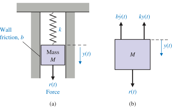
fig 2.1 (a) Spring-mass-damper system. (b) Free-body diagram.

Summing the forces acting on \(M\) and utilizing Newton’s second law yields

\[ M\frac{d^{2}y(t)}{dt^{2}} + b\frac{dy(t)}{dt} + ky(t) = r(t) \tag{2.1} \]

\(k\) is the spring constant of the ideal spring \(b\) is the friction constant. \(M\) is the mass of the brick \(y\) is the position of the brick (input) \(r\) is the resaltant force on the brick (output)

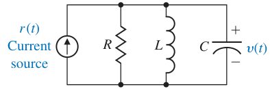
fig 2.2 RLC circuit

One may describe the electrical RLC circuit of fig 2.2 by utilizing Kirchhoff’s current law. Then we obtain the following integrodifferential equation:

\[ \frac{v(t)}{R} + C\frac{dv(t)}{dt} + L\int_0^t{v(t)dt} = r(t) \tag{2.2} \]

To reveal further the close similarity between the differential equations for the mechanical and electrical systems, we shall rewrite Equation (2.1) in terms of velocity:

\[ v(t) = \frac{dy(t)}{dt} \]

Then we have:

\[ M\frac{dv(t)}{dt} + bv(t) + k\int_0^t v(t)dt = r(t) \tag{2.3} \]

One immediately notes the equivalence of Equations (2.3) and (2.2) where velocity \(υ(t)\) and voltage \(υ(t)\) are equivalent variables, usually called analogous variables, and the systems are analogous systems.

2.3 Linear approximations of physical systems